Timing analysis
Timing analysis
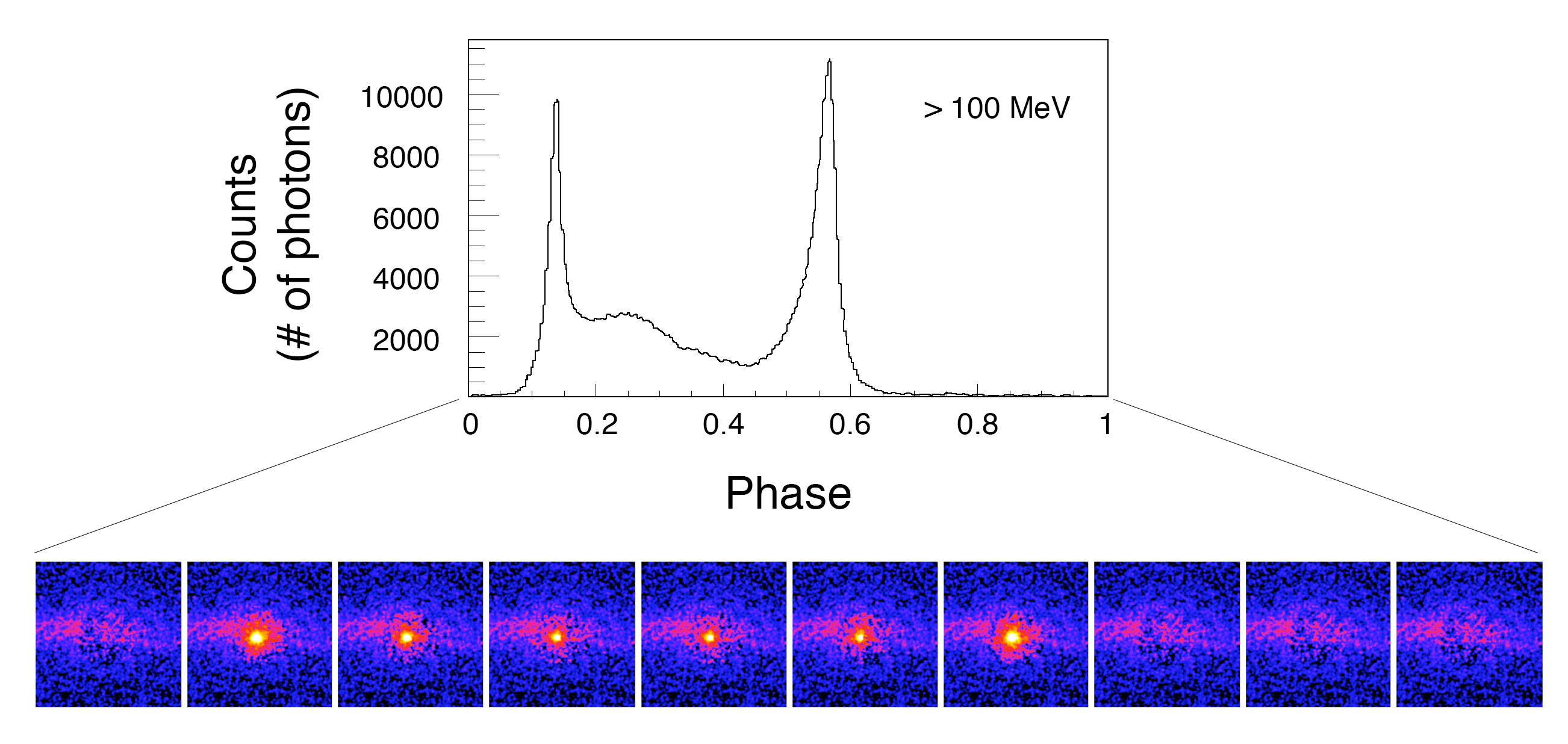
This figure shows time-lapse images of the Vela pulsar (bottom) and how they translate into a light curve (top). (Credit: Grodin et al. 2013 ApJ (light curve); NASA/DOE/Fermi LAT Collaboration (time lapse images))
Timing analysis allows astronomers to study the dynamic properties of an object. The targets of timing studies include accretion flows, oscillations, and accretion disk instabilities, as well as magnetic field configurations and instabilities in compact and non-compact stellar systems and active galaxies.
Anyone who has played a musical instrument knows how important it is to tune the instrument. Occasionally, a tuning fork is used to do that. A typical tuning fork used by musicians is for a pure A tone, of 440 Hz. But how does that apply in this situation? One Hertz (Hz) is one wave, or cycle, per second. A pure tone like an A travels just like a wave through the air, received by the eardrum as a signal at 440 waves per second. Now, imagine a musical chord. A C-major chord is made up of the notes C, E and G. The chord can be decomposed into three waves, each having a different frequency in Hz. In fact, any sound can be decomposed into a number of frequencies — some stronger, some weaker.
Sound is not the only type of data that can be decomposed into a number of frequencies. Astronomers can make time series data of astronomical objects. A time series is a series of data points taken at successive time intervals – data taken over time. Astronomers use a number of tools to study time series data in terms of the frequencies present in the data. This is useful to astronomers because it allows them to determine periodic components of the data, which can then be related to physical properties of the system, like rotation, binary period, and so on.
Methods of timing analysis
Fourier transform
A Fourier transform is a mathematical operation that changes data from time domain to frequency domain. This allows the data to be represented as the sum of a series of sines and cosines at various amplitudes, rather than as a continuous function.
Astronomers use Fourier transform to visualize the data as a large number of periodic components, each with a different period and a different strength. Very strong components may appear in data where there is a periodicity present. Astronomers then must estimate the significance of this feature (which is another way of saying that they must determine how much confidence they have that it is a true periodicity in the data).
When astronomers are looking for new phenomena, such as pulsars, they are very conservative in what they take to be a real signal. A frequency has to be many times stronger than it would be in a random data set to be taken seriously. A Fourier transform is based on a mathematical theorem that any signal can be decomposed into an infinite number of sine waves. This means that Fourier analysis works best when the signal we are looking for is very similar to a sine wave.
Fourier analysis of the time series on the left results in the Fourier power spectra on the right. It is clear that the analysis does identify the periodic behavior in the data.
Epoch folding
Another method that is useful for a signal with arbitrary shape is epoch folding. This is done by choosing a range of periods, and "folding" the data at those periods.
As an example, say an astronomer has one reading per second for 500 seconds of an object. She suspects that the object has a period of 25 seconds, so she will "fold the data on a period of 25 seconds." To do this, she would start with the first 25 points, and then add the second 25 points (points 26-50) to the first 25. Now add the third set of 25 points, and so on, until she reaches the end of the data set. If the period of the source is not close to 25 seconds, then times where the signal is high will cancel out with times where the signal is low in each of the 25 "bins", and the resulting epoch folded light curve will look sort of flat and boring. If, however, 25 seconds is very close to a period that is actually in the data, then bins where the signal is high will add together, and bins where it is low will add together, and the result will be a very nice looking epoch folded light curve. At this point, the astronomer must again assess how significant the resulting light curve is. This is generally done by looking at the spread of values, or errors, in the typical bin, and comparing how much higher the high bins are than the standard error.
The illustrations below show the process of epoch folding for an X-ray binary system called Circinus X-1 using data from the All-Sky Monitor aboard the RXTE satellite.
Here is the original lightcurve. There are spikes in the intensity that seem to repeat at regular intervals.
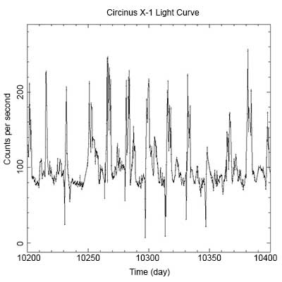
Light curve of X-ray binary system Circinus X-1. (Credit: NASA's Imagine the Universe.)
Looking closer at the data, we can determine that those peaks are occurring about every 16.6 days. So, let's cut the light curve into segments that are 16.6 days long.

Light curve of X-ray binary system Circinus X-1 cut into 16.6 day segments. (Credit: NASA's Imagine the Universe.)
To perform the epoch folding technique, we add those light curves together to end up with a single light curve that is 16.6 days in length where the intensities in each time bin are are the sum of the intensities of the cut lightcurves. If we've chosen a period that's close the real period, the highs will sum together to show a peak in the plot.
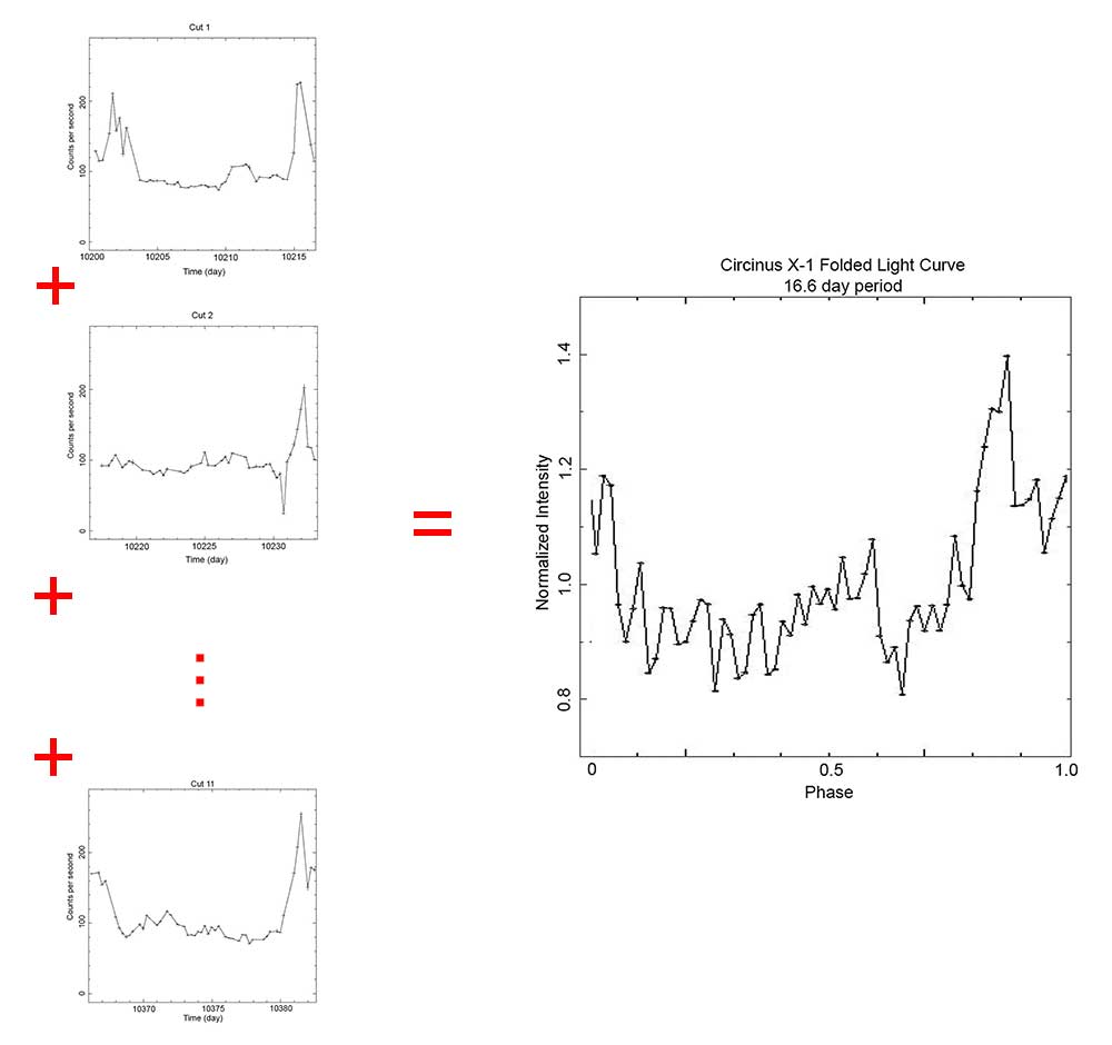
Illustration of the epoch folding technique. The individual 16.6-day light curves are summed into a single light curve covering just 16.6 days. If the chosen period is close to the period of variation for the object, the folded light curve will show an exaggerated peak. (Credit: NASA's Imagine the Universe.)
If we had picked a period that was not close to the period of the system, we would not have seen the peak in the summed light curve. Below are two "folded" lightcurves – the first is the one we just obtained using a 16.6 day period, the second is one made using a 10.5 day period. Notice that the 10.5 day period one does not show a strong peak, but is instead rather noisy. This tells us that the 10.5 day period is not close to the real period of the system.
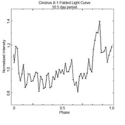
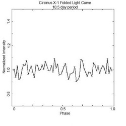
Two folded light curves for Circinus X-1. On the left, the folding period used was 16.6 days, which is close to the real period of the system. On the right, the folding period used was 10.5 days, quite different from the real period of the system. (Credit: NASA's Imagine the Universe.)
Wavelet analysis
Fourier transforms are great at finding systems that have a consistent periodicity, like pulsars. However, many sources of interest have periodic signals that vary over time, while other sources have many frequencies present in their data. For sources like this, wavelet analysis is used. Wavelet analysis also decomposes a signal into time and frequency space simultaneously.
Wavelet analysis is used primarily on signals where there are many frequencies, that may change with time, present in a data set. Both the epoch folding and the Fourier techniques tell you only about what frequencies are present in an entire data set, but nothing about how the strengths or values of these frequencies may change with time. Wavelet analysis is designed to capture time-varying frequencies and display them. Since more information is available than was gained from Fourier or epoch folding techniques, we need to represent the results of wavelet analysis differently. This is usually done in the form of an image that shows what frequencies were present at what times in the data set. While wavelet techniques are very powerful in helping astronomers uncover complex non-stationary behavior in data sets, they must be used with caution. The extra information that can be gained comes at the cost of increased difficulty in evaluating whether the result is significant. However, the fact that many of the most intriguing astronomical data sets appear to contain time varying frequency components demands that astronomers use every tool in their time series analysis toolbox, including wavelets.
Updated: August 2013