

GRB Distribution Across the Sky:
The Plots Thicken
Student Handout
Please read the following and answer the 18 questions given.
The discovery of GRBs was quite a shock to astronomers. Gamma rays are very high-energy photons, and it takes extremely energetic events to generate them. After all, GRBs were discovered when satellites were used to look for nuclear bomb tests on Earth! For GRBs to come from astronomical objects means they have to be extraordinary events. What kind of object could be at the heart of these phenomena?
One key to understanding GRBs is to know just how much energy they are emitting, and the only way to know that is to find their distance. The problem is, the flash of gamma rays lasts literally seconds, and in the early years of GRB astronomy there was no way known to determine their distance. The only physical characteristics astronomers were able to ascertain were the light curve of the flash of gamma rays (see Activity 1), and the direction to the GRB in the sky (see Activity 2).
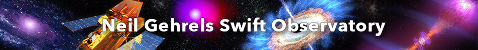
However, astronomers rapidly understood that the positions of the GRBs might give an important clue to understanding their physical nature. As a simple example, imagine you are standing in a field at night, and there are fireflies out. If you are in the middle of the field, the fireflies will be all around you, and you might correctly surmise you are in the middle of the field, even though you cannot see the borders. If, however, you are near the edge of the field, you will see more fireflies in one direction (towards the center of the field) than the other (toward the near edge). In the latter case, you can deduce that you are not in the center of the field because of the off-center pattern of lights.
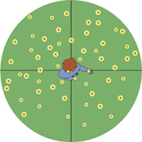
Figure 1
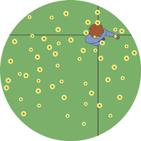
Figure 2
Figure 3
It would help even more to divide up your view into regions to aid counting; for example, you could use four quadrants, counting all the fireflies that are in the region from due north to due west, then due west to due south, etc. You could further subdivide to look for more detail, dividing each quadrant into 2 smaller sections, for example, for a total of 8 sections as in figure 3. This would allow a quantitative analysis of the distribution.
Gamma-ray bursts are far enough away that we cannot measure their distances directly. When GRBs were discovered, astronomers weren't sure if they were nearby (like in our solar system), very far away (like outside our galaxy), or at some intermediate distance (like inside our Milky Way Galaxy).
However, clever scientists realized that even if they couldn't measure the distance to GRBs, they could infer their distance, at least well enough to know if one of the choices above (near, middle or far) was wrong. They did this by looking at the distribution of GRBs in the sky.
The same is true for gamma-ray bursts. As more and more were detected, it became clear that they were distributed evenly across the sky. Even after careful examination by astronomers who divided the sky into many different bins, there was no apparent GRB clumping or voids in any directions, meaning they were truly in every direction in the sky. This immediately tells us that they are either very close or very far. Why?
Step 1: Having a Ball
In this activity, you will be looking at the distribution of aluminum foil balls arranged in a circle on the floor, and comparing them to the distribution of gamma-ray bursts on the sky. Your teacher will have already set up the circle of foil balls. Note the wedges dividing the circle into evenly spaced bins.
- How many balls are there in total?
- Given the diameter of the circle, what should the distance be between each ball (to the nearest 0.1 cm)?
- How many wedges are there?
- What is the angle covered by each pie wedge?
- On average, how many balls do you expect to find in each pie wedge?
Step 2: The Cutting Wedge
The wedges are centered on the center of the circle. We'll call this "Position 1". Count the number of balls in each pie wedge, filling out the table in the student worksheet as you do so.
When everyone is done filling out the table, move the wedge assembly so that the center of the wedges is located about halfway between the center of the circle of balls and the edge. Call this "Position 2".
- Do you expect to see the same distribution of balls in the wedges as you found before? Describe what you expect.
As before, count up the balls in each wedge, filling out the second table in the student worksheet.
On your graph paper, plot the number of balls you counted in each wedge versus the wedge number. Use dots for the first table (Position 1), and "x" for the second (Position 2). Draw "the line of best fit", a freehand curve that roughly follows the points (in other words, don't just connect the dots).
- In your own words, describe the two curves. How are they similar, different?
- The plot for Position 1 should ideally be perfectly flat, with the same number of balls in each wedge. However, your plot will not look like that. What is (are) the source(s) of deviation from a flat line?
- Calculate the total number of balls for both tables by summing up the numbers in the second column.
- Do these numbers surprise you? Why or why not?
- Calculate the average number of balls per wedge for both tables.
- Do these numbers surprise you? Why or why not? How do these numbers compare to what you calculated in Question 5?
Step 3: A Twist in the Plot
Now you will compare what you have found with real and simulated gamma-ray burst distributions in the sky. Figures 4 and 5 show computer-generated simulations of what the positions on the sky of gamma-ray bursts would look like if the GRBs had two different three-dimensional distributions.
Take a moment to examine them. Remember: these simulate the positions of the gamma-ray bursts on the sky, and show the entire sky.
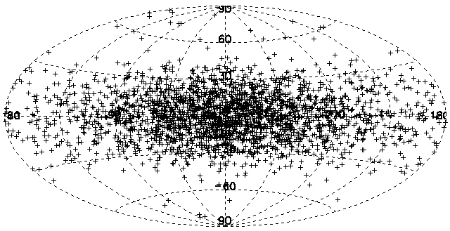
Figure 4
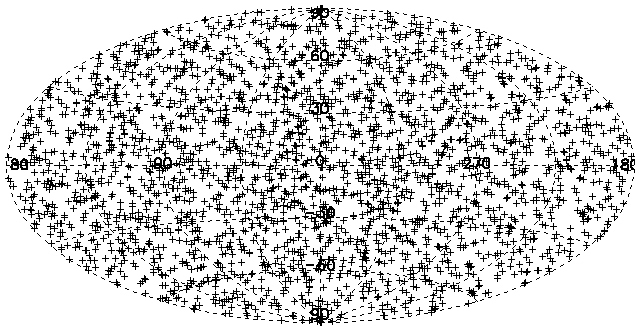
Figure 5
- In what ways are the plots similar? In what ways are they different? Be specific.
These plots are different than what you did before with the aluminum foil balls in that they show the distribution of GRBs over the area of the sky, whereas the foil balls were constricted to the circumference of a circle. To make comparison more useful, Figure 6 is a plot of the totals of the distribution from Figure 4 collapsed down to a line along the equator of the plot). Figure 7 is the same, but using the distribution from Figure 5.
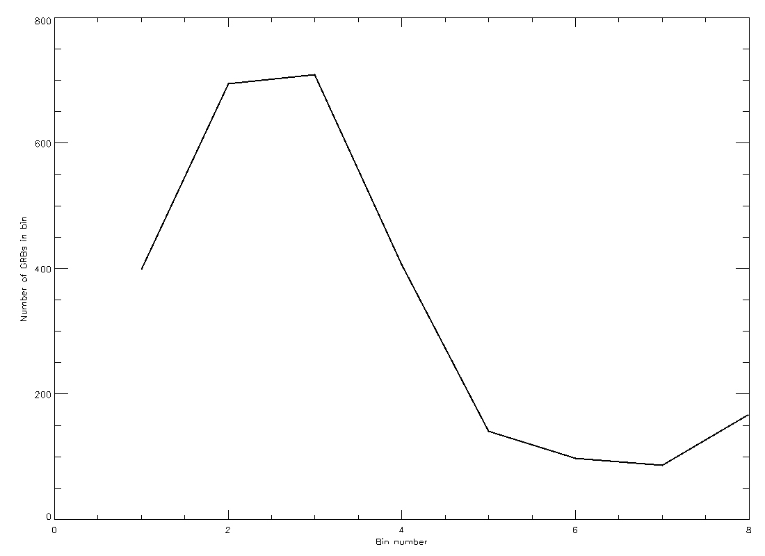
Figure 6
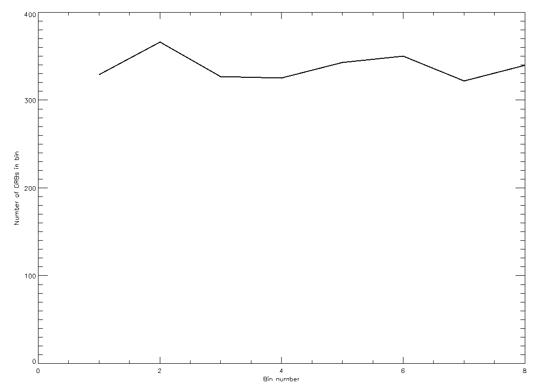
Figure 7
- Compare the plots you made using the aluminum foil balls for positions 1 and 2 with the Figure 6 and 7. Which figure looks more like your plot for the dot grid at position 1? Which looks like the plot for position 2?
The maps of the GRB positions in Figures 4 and 5 were generated using computer simulations assuming the GRBs were distributed a certain way in space.
- By comparing the plots to your own, describe in your own words how you think the GRBs were distributed in space for Figure 4 and Figure 5.
Step 4: BATSE in the Belfry
Figure 8 shows the real gamma-ray burst distribution in the sky, taken by NASA's Burst Alert and Transient Source Experiment (BATSE) detector that orbited the Earth from 1991 to 2000. There are 2704 bursts plotted on the map. Figure 9 shows the same thing, but collapsed down to a plane like Figures 6 and 7.
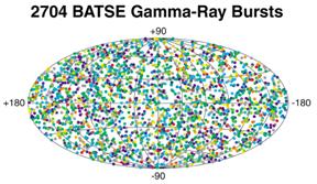
Figure 8
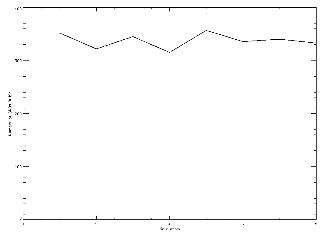
Figure 9
Compare the real distribution in the BATSE map to Figures 4 and 5, and the plot in Figure 9 to those in Figures 6 and 7.
- Which simulated distribution looks most like the real one? Does the collapsed plot match as well?
- What does this tell you about the real distribution of GRBs in space?
- Describe what this exercise tells you about determining the distance to GRBs.